Hénon map

The simplest use of MappyDS: a map that is discrete from the start. The Hénon map

\[x_{k+1} = 1 - a x_k^2 + y_k, \qquad y_{k+1} = b x_k\]

is declared as a Mapping and wrapped in a Diffeomorphism. With the classical values $a = 1.4$, $b = 0.3$ the orbit settles on the Hénon strange attractor. Python counterpart: examples/henon.py of mappy-ds.

using MappyDS, CairoMakie, StaticArrays
using MappyDS: image  # Makie exports an `image` plot function as well

henon = Mapping(2; name = :henon) do y, p
    x, u = y
    return SVector(1 - p.a * x^2 + u, p.b * x)
end
hmap = Diffeomorphism(henon)

params = (a = 1.4, b = 0.3)
y0 = [0.1, 0.1]

2-element Vector{Float64}:
 0.1
 0.1

Orbit

image applies the map once; iterating it collects the points of an orbit on the attractor.

function orbit(map, y0, params, n)
    points = Matrix{Float64}(undef, 2, n)
    y = y0
    for i in 1:n
        y = image(map, y, params)
        points[:, i] = y
    end
    return points
end

points = orbit(hmap, y0, params, 5000)
fig = Figure(; size = (600, 400))
ax = Axis(fig[1, 1]; xlabel = "x", ylabel = "y", limits = (-1.5, 1.5, -0.5, 0.5))
scatter!(ax, points[1, :], points[2, :]; markersize = 2, color = :teal)
fig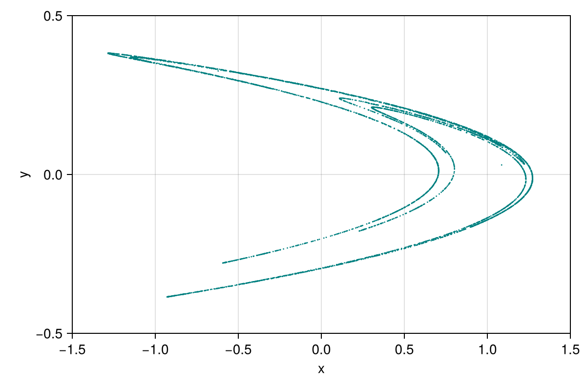

The same picture is produced by plot2d with a fixed number of frames (the viewer draws one image point per frame; only_map suppresses the jumps between successive points):

config = PlotConfig(;
    xlim = (-1.5, 1.5), ylim = (-0.5, 0.5), xlabel = "x", ylabel = "y",
    only_map = true, point_style = LineStyle(; color = :teal, alpha = 1.0),
    markersize = 2.0, param_keys = [:a, :b],
)
plot2d(hmap, y0, params, config; frames = 500, show = false)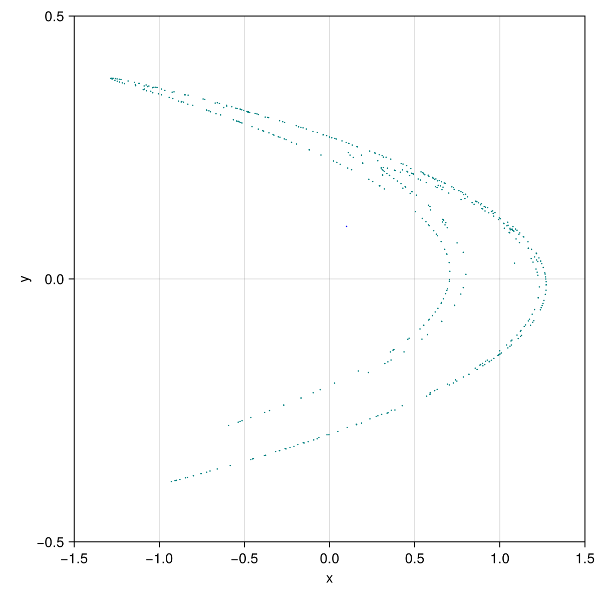

With GLMakie instead of CairoMakie the figure keeps iterating and reacts to the user: click to restart from a new initial point, f toggles the jumps between successive points, p switches between a and b and the up/down keys change the selected parameter.

using GLMakie
plot2d(hmap, y0, params, config)

Bifurcation diagram

Sweeping $a$ over $[1, 1.42]$ and recording $x$ after a transient gives the one-parameter bifurcation diagram (Miino 2024, Fig. 10, top). The state is carried over from one value of $a$ to the next.

a_range = (1.0, 1.42)
y_sweep = [-1.06770401965, 0.368194183333]  # on the attractor at a = 1.42

function bifurcation_diagram(map, params, a_values, frames)
    transient = frames ÷ 4
    xs = Matrix{Float64}(undef, frames - transient, length(a_values))
    y = y_sweep
    for (k, a) in enumerate(a_values)
        p = merge(params, (a = a,))
        for i in 1:frames
            y = image(map, y, p)
            i > transient && (xs[i - transient, k] = y[1])
        end
    end
    return xs
end

a_values = range(a_range...; length = 400)
xs = bifurcation_diagram(hmap, params, a_values, 400)
fig = Figure(; size = (800, 400))
ax = Axis(fig[1, 1]; xlabel = "a", ylabel = "x", limits = (a_range..., nothing, nothing))
scatter!(ax, repeat(collect(a_values); inner = size(xs, 1)), vec(xs); markersize = 1, color = :orange)
fig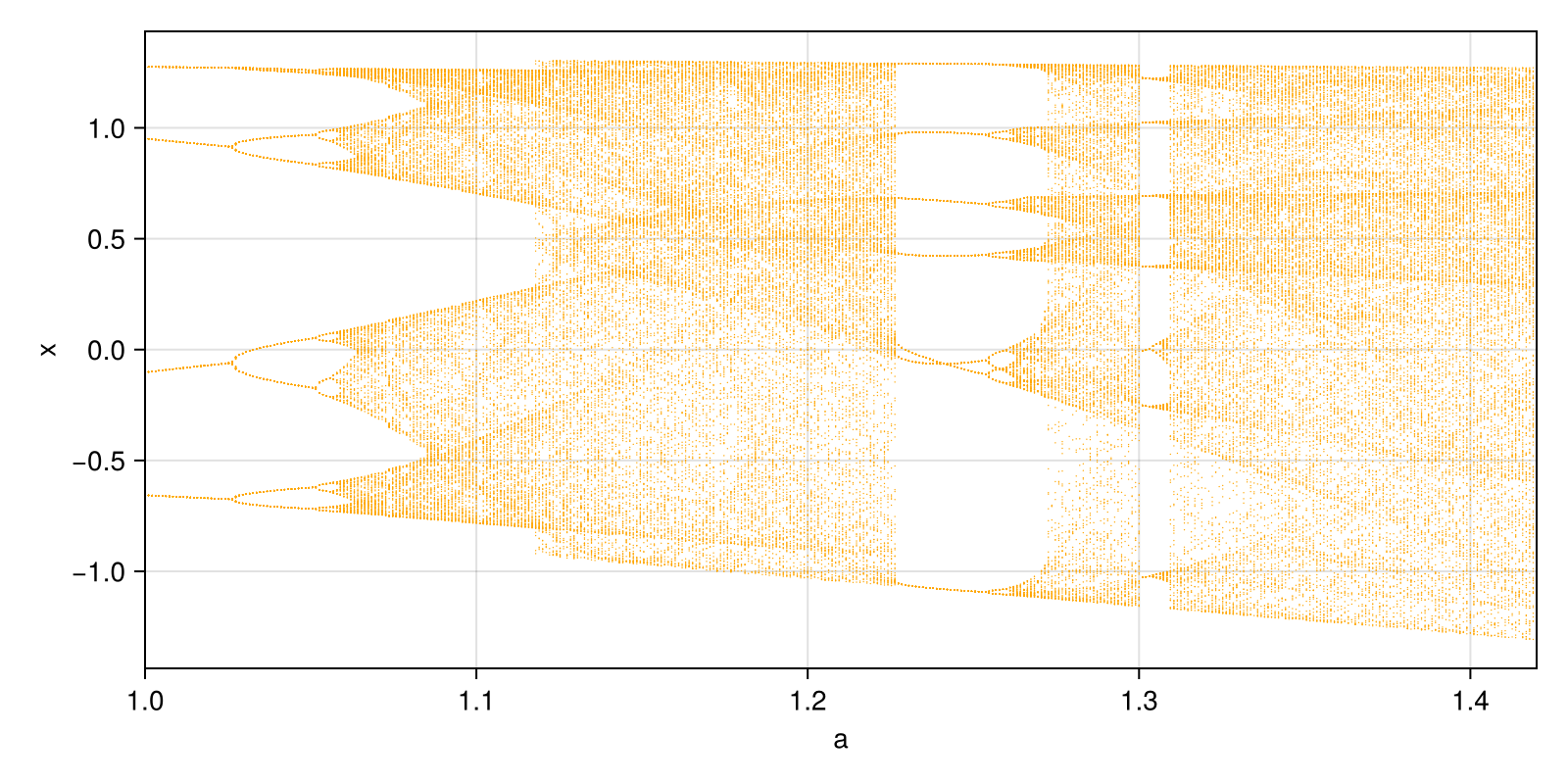

Maximum Lyapunov exponent

Benettin's method uses the Jacobian returned by image_detail: a unit tangent vector is pushed forward by res.jac at every iteration and renormalised, and the exponent is the mean of the logarithmic growth factors. It is positive exactly in the chaotic windows of the diagram (Miino 2024, Fig. 10, bottom).

function lyapunov(map, params, a_values, frames)
    mle = Float64[]
    y = y_sweep
    for a in a_values
        p = merge(params, (a = a,))
        unit = [1.0, 0.0]
        total = 0.0
        for _ in 1:frames
            res = image_detail(map, y, p)
            y = res.y
            unit = res.jac * unit
            growth = sqrt(sum(abs2, unit))
            total += log(growth)
            unit ./= growth
        end
        push!(mle, total / frames)
    end
    return mle
end

mle = lyapunov(hmap, params, a_values, 400)
fig = Figure(; size = (800, 300))
ax = Axis(fig[1, 1]; xlabel = "a", ylabel = "MLE", limits = (a_range..., nothing, nothing))
hlines!(ax, [0.0]; color = :gray, linewidth = 0.8)
lines!(ax, collect(a_values), mle; color = :red, linewidth = 1)
fig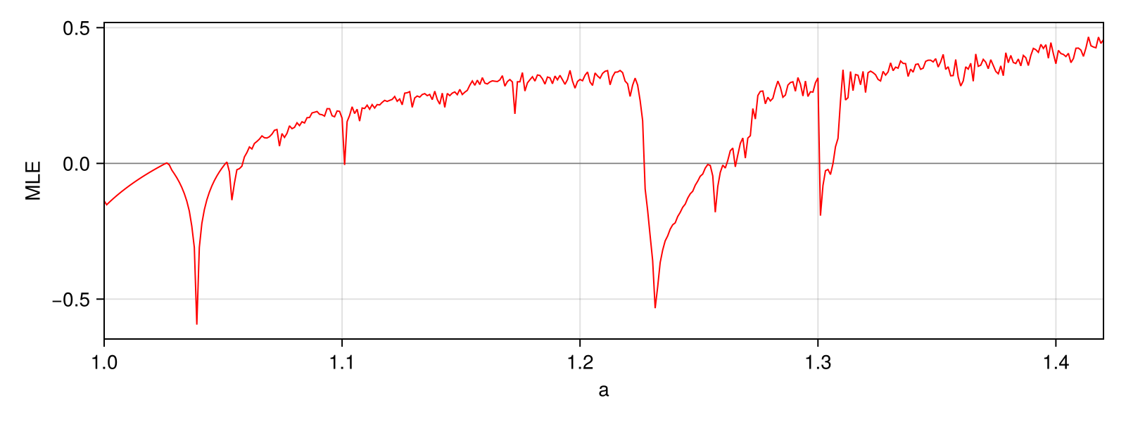

This page was generated using Literate.jl.